


It has been used in many ways and the paper itself has be very extensively cited.
Examples include:
- Plant and animal pathogen recognition receptors signal through non-RD kinases.
- Global target profile of the kinase inhibitor bosutinib in primary chronic myeloidleukemia cells
- Kinase binding selectivity for representative inhibitors shown on the human kinome dendrogram
If you are interested, please test the code and make comments. This is an ongoing project and I welcome feedback.
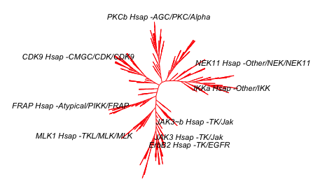
So here is the first version of the kinome phylogenetic tree:

I have made a more simple phylogenetic tree of the human proteins with the rel homology domain here which talks about the complexity of making trees.
Here is the script that makes this:
SCRIPT START
library(seqinr)
library(msa)
library(ape)
# first version of generating a the kinome visualisation in R
# data is here: http://kinase.com/kinbase/FastaFiles/Human_kinase_domain.fasta
# in fasta format...
# need to extract the data into R...
# need Biostrings package - downloaded as part of seqinr package
file <- c("http://kinase.com/kinbase/FastaFiles/Human_kinase_domain.fasta")
# step 1 is read in the FASTA files.
kinases <- readAAStringSet(file, format = "fasta")
# that seems to work.
kinases
# 516 sequences.
# good.
# step 2 do the multiple sequence alignment
kinaseAlign <- msa(kinases)
# takes a bit of time! - about 3.5 min on my computer...
# currently using default substitution matrix and CLUSTALW
# creates an object with Formal class 'MsaAAMultipleAlignment' [package "msa"] with 6 slots
# step 3: convert Msa Alignment object into alignment for seqinr
kinaseAlign2 <- msaConvert(kinaseAlign, type="seqinr::alignment")
class(kinaseAlign2) # it's an alignment
# worked
# List of 4
# step 4: compute distance matrix - dist.alignment() function from the seqinr package:
d <- dist.alignment(kinaseAlign2, "identity")
# Class 'dist'
kinaseTree <- nj(d) # from ape package, I think...
class(kinaseTree)
# class "phylo"
# List of 4
# good idea to save the tree locally... remove comment symbol
# write.tree(kinaseTree, file = "kinaseTree")
# to read back in:
# kinaseTree <- read.tree(file = "kinaseTree")
plot(kinaseTree,
main="Phylogenetic Tree of kinases")
# too difficult to read so remove the tip.labels which are the kinase names.

plot(kinaseTree,
main= "Phylogenetic Tree of kinases",
show.tip.label = FALSE)

type = "unrooted",
main= "Phylogenetic Tree of kinases",
show.tip.label = FALSE)

# looks quite stylish a a little similar to visualisation in the Science paper
plot(kinaseTree, "u",
use.edge.length = FALSE,
show.tip.label = FALSE)

# need to add colour
# argument is edge.color
plot(kinaseTree, "u",
use.edge.length = FALSE,
show.tip.label = FALSE,
edge.color = "red")

# want to add selected labels to give some orientation
# extract tip.labels
tipLabels <- kinaseTree$tip.label
# add some labels we like to orient ourselves:
kinaseLabels <- c("IKKa","JAK3","ErbB2",
"NEK11", "MLK1", "PKCb",
"CDK9", "FRAP")
# find these in the alignment - they will be tip labels
labelNo <- NULL
for(i in 1:length(kinaseLabels)){
labelNo <- c(labelNo, grep(kinaseLabels[i], kinaseTree$tip.label))
}
# generates a vector of 9 numbers. Some labels in two names.
# make a vector of blank tiplabels
tipLabels_2 <- rep('', length(kinaseTree$tip.label))
# add the labels we want to the vector...
for(i in 1:length(labelNo)){
tipLabels_2[labelNo[i]] <- tipLabels[labelNo[i]]
}
# make a new tree
kinaseTree_fewLabels <- kinaseTree
# replace the tip labels with the shorter list.
kinaseTree_fewLabels$tip.label <- tipLabels_2
# make the plot with these
plot(kinaseTree_fewLabels, "u",
use.edge.length = FALSE,
show.tip.label = TRUE,
edge.color = "red",
cex = 0.7)
# remove "Hsap" using gsub() function
tipLabels_2 <- gsub("Hsap", "", tipLabels_2)
kinaseTree_fewLabels$tip.label <- tipLabels_2
plot(kinaseTree_fewLabels, "u",
use.edge.length = FALSE,
show.tip.label = TRUE,
edge.color = "red",
cex = 0.7)

# add a title and source and you have the image at the top...
plot(kinaseTree_fewLabels, "u",
main="Phylogenetic tree of human kinase domains",
sub="source: www.kinase.com & Manning et al Science (2002) 398:1912-1934",
use.edge.length = FALSE,
show.tip.label = TRUE,
edge.color = "red",
cex = 0.7)
# this looks quite good and is enough for today.
No comments:
Post a Comment
Comments and suggestions are welcome.