


I have been exploring the possibility of using R to open and analyse some images. This was first prompted by a delegate that attended our R for Biochemists Training Day organised through the Biochemical Society.
Our search revealed the Bioconductor package, EBImage which allows the opening of .jpg files using R. This allowed me to extract the fluorescence values that I had from this image which I prepared with a colleague, Dr Elisabeth Walsby. Beth stained the cell and I did the confocal microscopy. Here is the nice picture of a chronic lymphocytic leukaemia cell stained for a protein (red colour) and for DNA (blue).

I can open this image with R using the readImage() function that comes as part of the EBImage package. When I display the image using the display() command, it opens a new browser window. It has various functionality to explore the image shown here:

The most useful aspect of this approach is the ability to extract the fluorescence values to use to make nice plots in R. This uses the imageData() function which works like this:
- imageData(img)[, 512, 3] - access a vector with all the x values across one y value (pixel number 512) and extracts the third colour for the image.
I've used EBImage to extract values and to generate this graph which shows the fluorescence of the pixels across the middle of the cell:
Here is the script with some plots that I generated along the way:
# EBImage - a Bioconductor package for analysing images
source("http://bioconductor.org/biocLite.R")
biocLite("EBImage")
library("EBImage")
library(ggplot2)
# the image is on Github
img <- readImage("https://raw.githubusercontent.com/brennanpincardiff/RforBiochemists/master/data/images/cllCell.jpg")
# the object created is a Large Image (24 Mb in this case!)
img <- readImage("https://raw.githubusercontent.com/brennanpincardiff/RforBiochemists/master/data/images/cllCell.jpg")
# the object created is a Large Image (24 Mb in this case!)
display(img)
# opens a window in a web browser and allows you to look at the image
print(img)
# shows some of the structure of the Large Image object.
dim(img)
# [1] 1024 1024 3
# corresponds to x and y pixels of the image and then the number of colours for each pixel
# why do we want to do this?
# so that we can extract data out of the image and draw nice graphs.
# to extract a value out of the Large Image use the imageData() function
# if you place the mouse over the image in the web browser, you see the name of the pixel.
# we can extract the fluorescence value and plot the data
x <- imageData(img)[, 512, 3]
# this gives the values for colour 3 for the whole x line at the value of y = 512.
# this is a list of 1024 numbers which can be plotted
plot(x)

# the index at the bottom refers to the x values across the whole image.
# using the web browser, I can choose the line across the middle of the cell
# extract a row of 100 pixels wide from left to right of the middle of the image.
# I chose to extract values from y pixel 425 to 545 which correspond to the middle of the cell
# colour 1
x10.col1 <- as.data.frame(imageData(img)[ ,425:525, 1])
plot(x10.col1$V5) # plot one of the values
 |
| Plot one of the values (V5) |
x10.col1$mean <- rowMeans(x10.col1[1:100])
plot(x10.col1$mean) # plot the mean
 |
| Plot the mean of 100 pixels |
# colour 3
x10.col3 <- as.data.frame(imageData(img)[ ,425:525, 3])
x10.col3$mean <- rowMeans(x10.col3[1:100])
plot(x10.col3$mean, col = "blue")
lines(x10.col1$mean, col = "red")
 |
| Plot both colours using Base R |
# assemble a data frame to allow us to use ggplot to plot the data..
m <- as.data.frame(x10.col1$mean)
m$col3 <- x10.col3$mean
# change the column names in the data frame
colnames(m) <- c("col1", "col3")
# make the basic ggplot object
p <- ggplot(data=m, aes(x=seq(1, length(col3)))) +
geom_line(aes(y = col3), colour = "blue") +
geom_line(aes(y = col1), colour = "red")
p # show the plot
 |
| Plot both colours in ggplot2 |
# focus on just the cell
p <- ggplot(data=m, aes(x=seq(1, length(col3)))) +
geom_line(aes(y = col3), colour = "blue") +
geom_line(aes(y = col1), colour = "red") +
xlim(350,850) # focus on just the cell
p # have a look
# gives Warning messages but these can be ignored.
 |
| Focus on the cell by limiting the x-axis. |
# add some titles and a easy theme
p <- p + xlab("Distance (pixels)") + #label x-axis
ylab("Fluorescence signal") + #label y-axis
ggtitle("Histogram of fluoresence of CLL cell") + #title
theme_bw() # a simple theme
p # show the plot
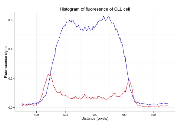 |
| Add titles and change the theme. |
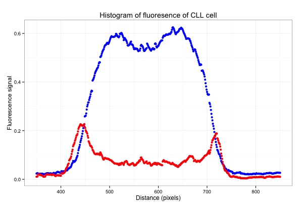
# plot points instead of lines...
q <- ggplot(data=m, aes(x=seq(1, length(col3)))) +
geom_point(aes(y = col3), colour = "blue") +
geom_point(aes(y = col1), colour = "red") +
xlim(350,850) +
xlab("Distance (pixels)") + # label x-axis
ylab("Fluorescence signal") + # label y-axis
ggtitle("Histogram of fluoresence of CLL cell") + # add a title
theme_bw() # a simple theme
q # show the plot
You have the plot at the top of the page....
Resources:
- My first link to EBImage: http://www.r-bloggers.com/r-image-analysis-using-ebimage/
- Introduction to EBImage (PDF): http://bioconductor.org/packages/release/bioc/vignettes/EBImage/inst/doc/EBImage-introduction.pdf
- Reference manual for EBImage: http://bioconductor.org/packages/release/bioc/manuals/EBImage/man/EBImage.pdf
- http://www.cookbook-r.com/Graphs/Axes_(ggplot2)/
- http://stackoverflow.com/questions/13837565/how-to-plot-one-variable-in-ggplot
No comments:
Post a Comment
Comments and suggestions are welcome.